The manifold art of Conrad Shawcross

2018-04-16

by Andrie de Vries

During April, 2018, I went to visit the Whitechapel Art Gallery, a wonderful art gallery in the center of London.

One of the exhibits on display was a piece by Conrad Shawcross, as part of his exhibition on Art Capital: Art for the Elizabeth line that ran from 13 March to 6 May 2018.

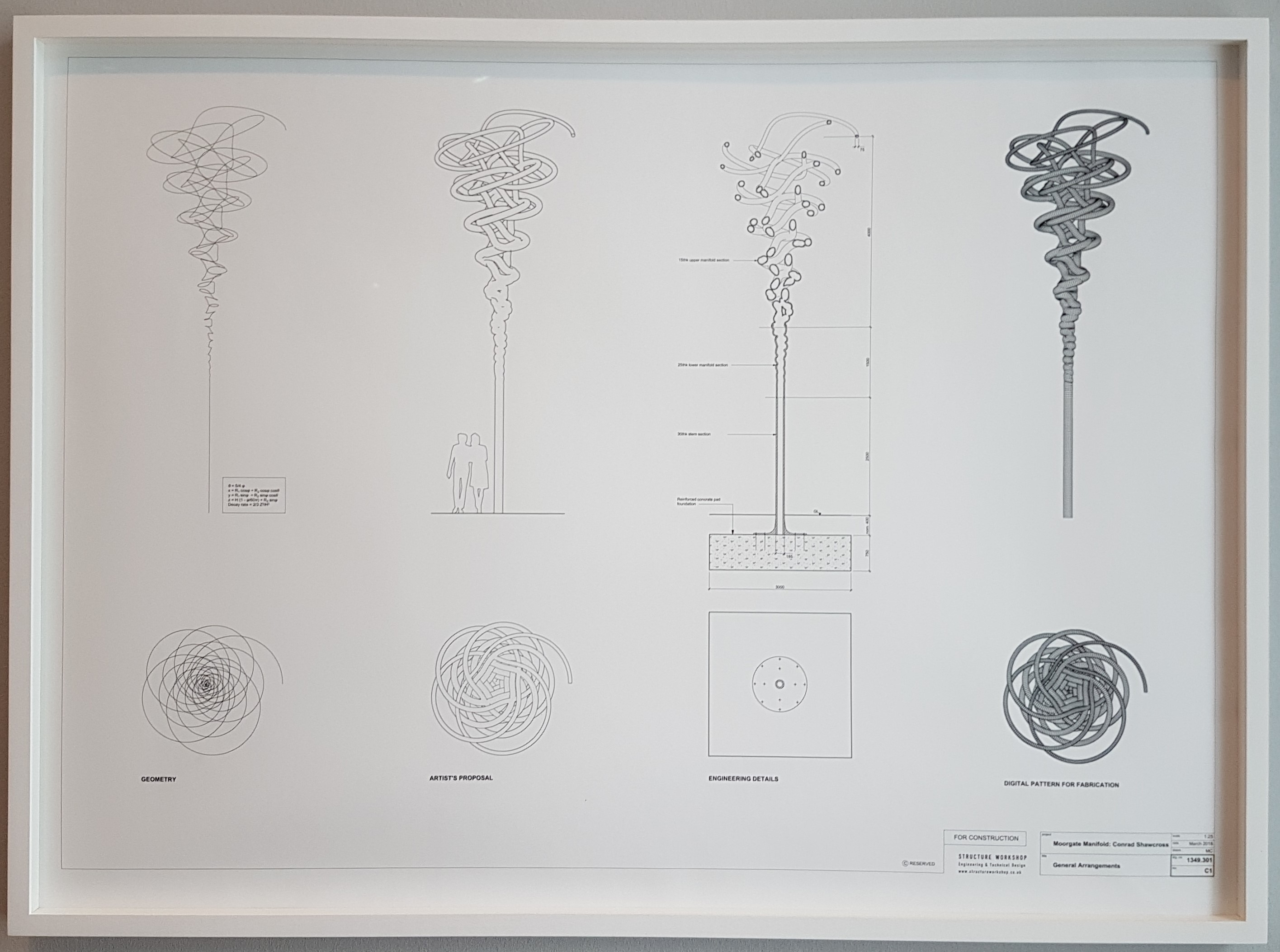
One of the pieces on display was design drawings of his “Manifold” sculpture that is positioned outside the Moorgate entrance of the Elizabeth line station in London.

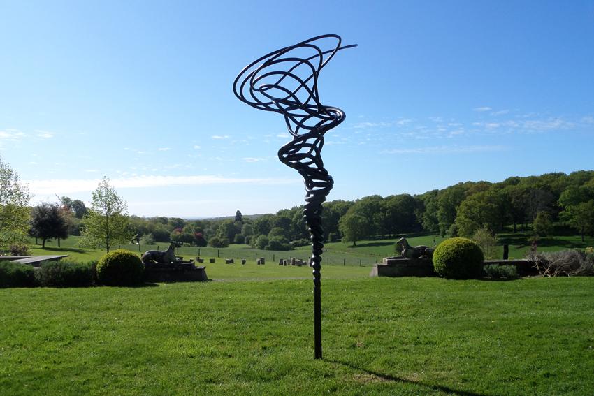
He has created a number of pieces in his manifold series, e.g. “Manifold 2 (9:8)” that was exhibited at the New Art Centre in Salisbury, Wiltshire:

At the Whitechapel exhibition, I took a picture of the design drawings for the “Moorgate Manifold”, that shows various views, including top, side and cutout views:

On close inspection I could see some equations in the drawing:

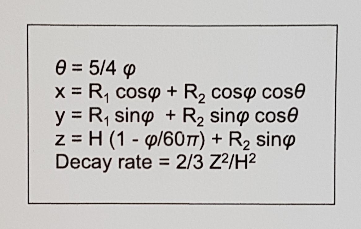
Clearly the original idea was based on a mathematical equation, so I set about trying to replicate this drawing using R code.

The code

My attempt at replicating the manifold, using code. I had to guess (by experimentation) the initial values of R1, R2 and H. I also had to guess that the decay rate is a function that only applies to the x and y dimensions.

manifold <- function(psi, R1 = 1, R2 = 0.5, H = 7){
  theta <- 5/4 * psi
  x <- R1 * cos(psi) + R2 * cos(psi) * cos(theta)
  y <- R1 * sin(psi) + R2 * sin(psi) * cos(theta)
  z <- H * (1 - psi / (60 * pi)) + R2 * sin(psi)
  
  decay <- function(x){
    x * 2/3 * z^2 / H^2
  }
  
  as.data.frame(cbind(
    x = decay(x),
    y = decay(y),
    z = z
  ))
}

Having defined the function, it is straight-forward to generate some values of the data.

x <- seq(0, 30 * 7, by = 0.01)
dat <- manifold(x)
head(dat)
##          x          y        z
## 1 1.000000 0.00000000 7.000000
## 2 1.001247 0.01001280 7.004629
## 3 1.002342 0.02004950 7.009257
## 4 1.003284 0.03010755 7.013884
## 5 1.004073 0.04018434 7.018509
## 6 1.004708 0.05027730 7.023133

Now you can plot the results. First, the view from the top down:

library(ggplot2)
ggplot(dat, aes(x = x, y = y, col = z)) + 
  geom_point(size = 0.1) + 
  coord_equal() + 
  scale_color_gradient(low = "grey80", high = "black") +
  theme_minimal()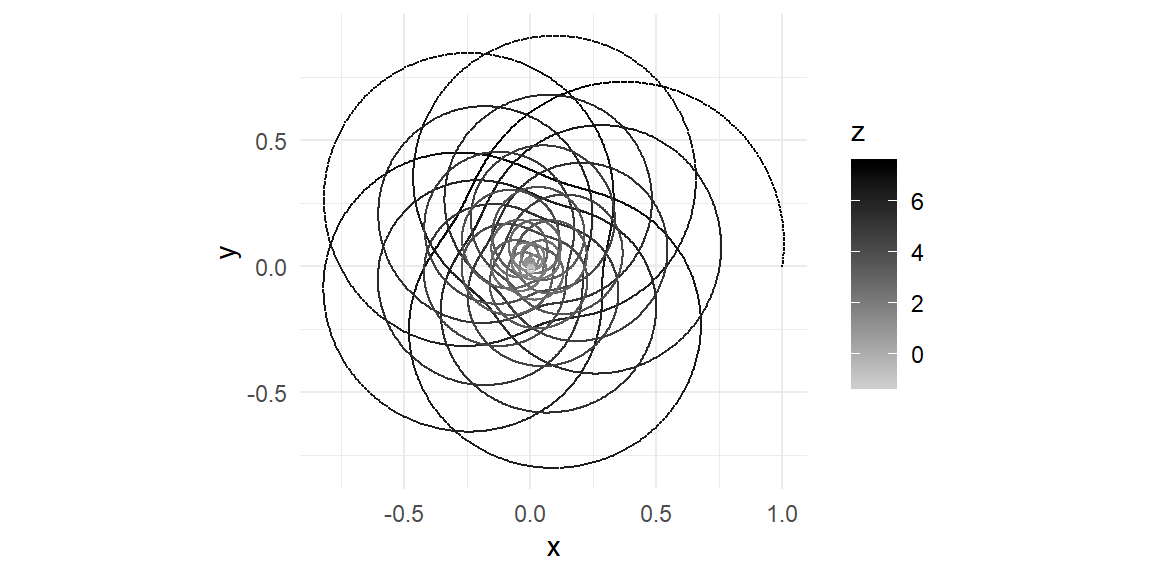

And next, a sideways view:

ggplot(dat, aes(x = z, y = x, col = y)) + 
  geom_point(size = 0.1) + 
  scale_color_gradient(low = "grey50", high = "black") +
  coord_equal() + 
  theme_minimal()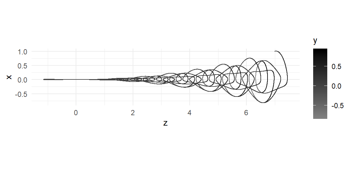

You can also use rgl to create an interactive 3D viewer. Note that you can rotate the object by clicking and dragging on the plot:

library(rgl)
with(dat, plot3d(x, y, z))

You must enable Javascript to view this page properly.